How to Assess Clustering Tendency: Unsupervised Machine Learning

The meaning of clustering algorithms include partitioning methods (PAM, K-means, FANNY, CLARA etc) along with hierarchical clustering which are used to split the dataset into two groups or clusters of similar objects.

A natural question that comes, before applying any clustering method on the dataset is:

Does the dataset comprise of any inherent clusters?

A big problem associated to this, in case of unsupervised machine learning is that clustering methods often return clusters even though the data does not include any clusters. Put in other words, if one blindly applies a clustering analysis on a dataset, it will divide the data into several clusters because that is precisely what they are supposed to do.

So, before selecting a clustering approach the analysts must decide whether the dataset includes meaningful clusters (which is non-random structures) or does not. And if there exists, then one must understand how many clusters exists in the set. This system is defined as the assessing o clustering tendency or the feasibility of the clustering analysis.

In this article, we will learn the following things:

• Describing why we should assess the clustering tendencies (also called as clusterability) before actually applying any cluster analysis on a particular dataset.
• We will also describe a statistical method for evaluating the clustering tendency.

Necessary packages:

The below mentioned R packages are needed to understand this post:

1. For visualization purposes factoextra
2. To evaluate the clustering tendency clustertend package
3. To visually assess the cluster tendency seriation package

One can install factoextra as follows:

if(!require(devtools)) install.packages("devtools")

devtools::install_github("kassambara/factoextra") 

To install seriation and clustertend, follow these steps: 

install.packages("clustertend") 

install.packages("seriation")  Loading the necessary packages, can be done through the following:

library(factoextra)

library(clustertend)

library(seriation)

Preparing the data:

We will use two datasets – the built-in R dataset called ‘faithful’ and another simulated dataset.

Using ‘faithful’ dataset:

The ‘faithful’ dataset consists of a waiting time, which is between eruptions and the duration of the eruption of the Old Faithful Geyser at Yellowstone National Park, in Wyoming USA!

# Load the data

data("faithful")

df <- faithful

head(df)

##   eruptions waiting

## 1     3.600      79

## 2     1.800      54

## 3     3.333      74

## 4     2.283      62

## 5     4.533      85

## 6     2.883      55

All the required illustrations can be made using ggplot2 package as follows:

library("ggplot2")

ggplot(df, aes(x=eruptions, y=waiting)) +

  geom_point() +  # Scatter plot

  geom_density_2d() # Add 2d density estimation

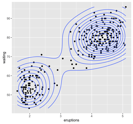
Image Source: r-bloggers.com

Random uniformly distributed dataset:

The R code mentioned below generates a random uniform data with the same dimension just like a faithful dataset. With the function, runif(n, min, max) which is used to generate uniform distribution on the interval of min to max.

# Generate random dataset

set.seed(123)

n <- nrow(df)

random_df <- data.frame(

  x = runif(nrow(df), min(df$eruptions), max(df$eruptions)),

  y = runif(nrow(df), min(df$waiting), max(df$waiting)))

# Plot the data

ggplot(random_df, aes(x, y)) + geom_point()

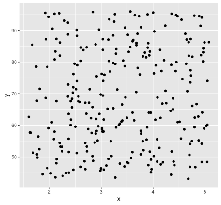
Image Source: r-bloggers.com

A noteworthy point here is that for a given real dataset, random uniform data may be generated within a single function call as can be shown below:

random_df <- apply(df, 2,

                function(x, n){runif(n, min(x), (max(x)))}, n)

The need to assess clustering tendency:

As mentioned above, we know that the ‘faithful’ dataset actually comprises of two real clusters. But the randomly generated dataset will not contain any meaningful cluster.

The below mentioned R code will help to compute, K-means clustering and/or hierarchical clustering on both the datasets. To visualize the results, we will use the function fviz_cluster() and fviz_dend() [in factoextra].

library(factoextra)

set.seed(123)

# K-means on faithful dataset

km.res1 <- kmeans(df, 2)

fviz_cluster(list(data = df, cluster = km.res1$cluster),

             frame.type = "norm", geom = "point", stand = FALSE)

To know more about clustering analysis, you can take up an R Programming Online Training with us at DexLab Analytics. We also offer classroom based R language training as well as in Gurgaon. Join us now…
 
This post originally appeared on – www.r-bloggers.com/assessing-clustering-tendency-a-vital-issue-unsupervised-machine-learning
 

Interested in a career in Data Analyst?

To learn more about Data Analyst with Advanced excel course – Enrol Now.
To learn more about Data Analyst with R Course – Enrol Now.
To learn more about Big Data Course – Enrol Now.

To learn more about Machine Learning Using Python and Spark – Enrol Now.
To learn more about Data Analyst with SAS Course – Enrol Now.
To learn more about Data Analyst with Apache Spark Course – Enrol Now.
To learn more about Data Analyst with Market Risk Analytics and Modelling Course – Enrol Now.