Basics of a Two-Variable Regression Model: Explained

In continuation of the previous Regression blog, here we are back again to discuss the basics of a two-variable regression model. To read the first blog from the Regression series, click here www.dexlabanalytics.com/blog/a-regression-line-is-the-best-fit-for-the-given-prf-if-the-parameters-are-ols-estimations-elucidate.

In Data Science, regression models are the major driver to interpret the model with necessary statistical methods, practically as well as theoretically. One, who works extensively with business data metrics, will be able to solve various tough problems with the help of a regression theory. The key insight of the regression models lies in interpreting the fitness of the models. But it differs from the standard machine learning techniques such that, for improvement in the performance of the model being predicted, the major interpretable coefficients are never sacrificed. Thus, a sense in regression models can be considered as the most important tool to be chosen for solving any practical problem.

Let’s consider a simple example to understand regression analysis from scratch. Say, we want to predict the sales of a Softlines eCommerce company for this year during the festivals of Diwali. There are a lot of factors to generate impacts on the sales value, as there are hundreds of factors persisting within the model. We can consider our own judgement to get the impacting factors. Now, here in our model, the value of sales that we want to predict is the dependent variable, whereas the impacting factors are considered as the independent variables. To analyse this model in terms of regression, we need to gather all the information about the independent variables from the past few years, and then act on it according to the regression theory.

Before getting into the core theory, there are some basic assumptions for such a two-variable regression model and they are as follows:

• Variables are linearly related: The variables in a 2-variable Regression Model are linearly related, the linearity being in parameters, though not always in variables, i.e. the power in which the parameters appear should be of 1 only and should not be multiplied or divided by any other parameters. These linearly related variables are basically of two types (i) independent or explanatory variables & (ii) dependent or response variables.
• Variables can be represented graphically: The idea behind this assumption guarantees that observations must be real numbers represented on graph papers.
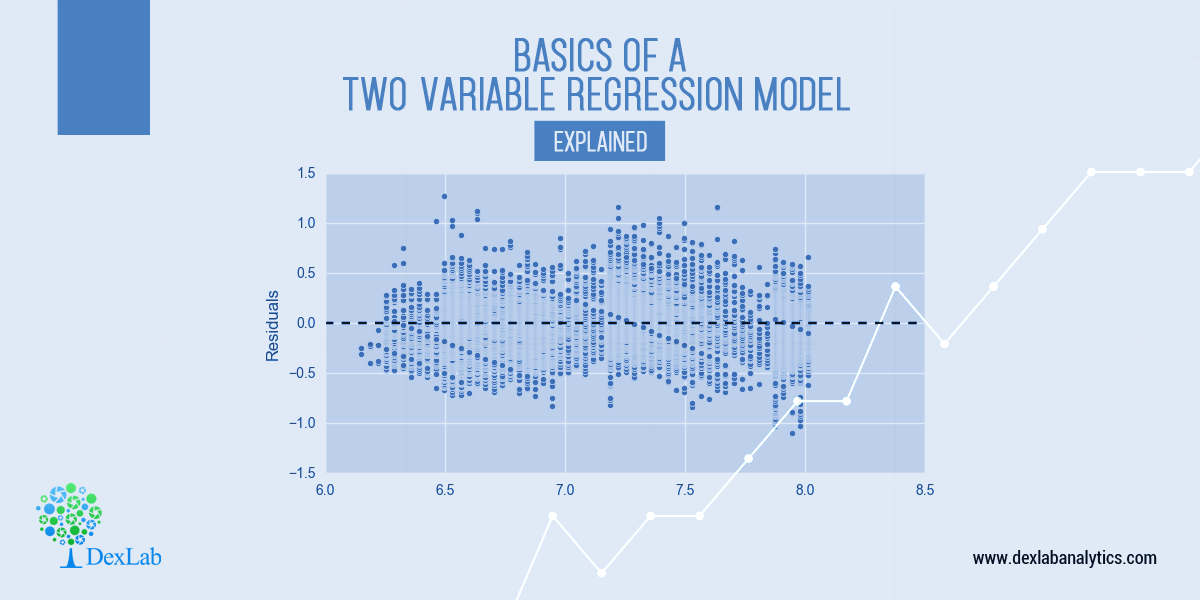
• Residual term and the estimated value of the variables are uncorrelated.
• Residual terms and explanatory variables are uncorrelated.
• Error variables are uncorrelated with mean 0 & common variance σ²

Now, how can a PRF for expanding an economic relationship between 2 variables be specified?

Well, Population regression function, or more generally, the population regression curve, is defined as the locus of the conditional means of the dependent variables, for a fixed value of the explanatory variables. More simply, it is the curve connecting the means of the sub-populations of Y corresponding to the given values of the regressor X.

Formally, a PRF is the locus of all conditional means of the dependent variables for a given value of the explanatory variables. Thus; the PRF as economic theory would suggest would be:

Where 9(X) is expected to be an increasing function of X, if the conditional expectation is linear in X. then

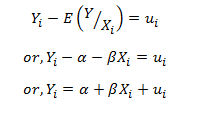
Hence, for any ith observations:

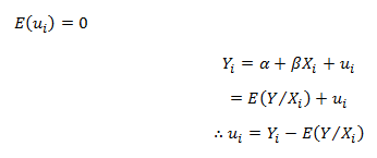
However, the actual observation for the dependent variable is Y_i. Therefore; Y_i – E(Y/X_i) = u_i, which is the disturbance term or the stochastic term of the Regression Model.

Thus,

…………………… (A)

• is the population regression function and this form of specifying the population regression function is called the stochastic specification of the PRF.

Stochastic Specification of the Model:

Y_i = α + βX_i + u_i is referred to as the stochastic specification of the Population Regression Function, where u_i is the stochastic or the random disturbance term. It explains everything’s net influence other than X variable on the ith observation. Thus, u_i is a surrogate or proxy for all omitted or neglected variables which may affect Y but is not included in the model. The random disturbance term is incorporated into the model with the following assumptions:-

Proof:

Taking conditional expectation as both sides, we get:

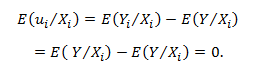
Hence; E(u_i) = 0

cov(u_i,u_j) = E(u_i u_j ) = 0 ∀ i ≠ j i.e. the disturbance terms are distributed independently of each other.

Proof:

Two variables are said to be independently distributed, or stochastically independent; if the conditional distributions are equal to the corresponding marginal distributions.

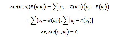
Hence; cov(u_i,u_j )= E(u_i u_j ) = 0 Thus, no auto correction is present among ui,s i.e. ui,s. s are identically and independently distributed Random Variables. Hence, ui,s are all Random Samples.

Proof:

The conditional variance between two error terms can be given as given independence &

All these assumptions can be embodied in the simple statement: u_i~N(0,σ²) where u_i,s are iid’s ∀ I, Which heads “the ui are independently distributed identically distributed with mean 0 & variance σ²”.

Last Notes

The benefits of regression analysis are immense. Today’s business houses literally thrive on such analysis. For more information, follow us at DexLab Analytics. We are a leading data science training institute headquartered in Delhi NCR and our team of experts take pride in crafting the most insight-rich blogs. Currently, we are working on Regression Analysis. More blogs are to be followed on this model. Keep watching!

Interested in a career in Data Analyst?

To learn more about Data Analyst with Advanced excel course – Enrol Now.
To learn more about Data Analyst with R Course – Enrol Now.
To learn more about Big Data Course – Enrol Now.

To learn more about Machine Learning Using Python and Spark – Enrol Now.
To learn more about Data Analyst with SAS Course – Enrol Now.
To learn more about Data Analyst with Apache Spark Course – Enrol Now.
To learn more about Data Analyst with Market Risk Analytics and Modelling Course – Enrol Now.