ARMA(p,q) model in time series forecasting is a combination of Autoregressive Process also known as AR Process and Moving Average (MA) Process where p corresponds to the autoregressive part and q corresponds to the moving average part.
![]()

Autoregressive Process (AR) :- When the value of Yt in a time series data is regressed over its own past value then it is called an autoregressive process where p is the order of lag into consideration.

Where,
Yt = observation which we need to find out.
α1= parameter of an autoregressive model
Yt-1= observation in the previous period
ut= error term
The equation above follows the first order of autoregressive process or AR(1) and the value of p is 1. Hence the value of Yt in the period ‘t’ depends upon its previous year value and a random term.
Moving Average (MA) Process :- When the value of Yt of order q in a time series data depends on the weighted sum of current and the q recent errors i.e. a linear combination of error terms then it is called a moving average process which can be written as :-
![]()

yt = observation which we need to find out
α= constant term
βut-q= error over the period q .
ARMA (Autoregressive Moving Average) Process :-

The above equation shows that value of Y in time period ‘t’ can be derived by taking into consideration the order of lag p which in the above case is 1 i.e. previous year’s observation and the weighted average of the error term over a period of time q which in case of the above equation is 1.
How to decide the value of p and q?
Two of the most important methods to obtain the best possible values of p and q are ACF and PACF plots.
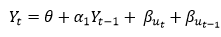
ACF (Auto-correlation function) :- This function calculates the auto-correlation of the complete data on the basis of lagged values which when plotted helps us choose the value of q that is to be considered to find the value of Yt. In simple words how many years residual can help us predict the value of Yt can obtained with the help of ACF, if the value of correlation is above a certain point then that amount of lagged values can be used to predict Yt.
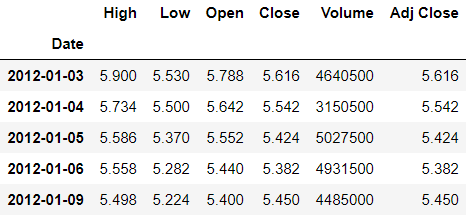
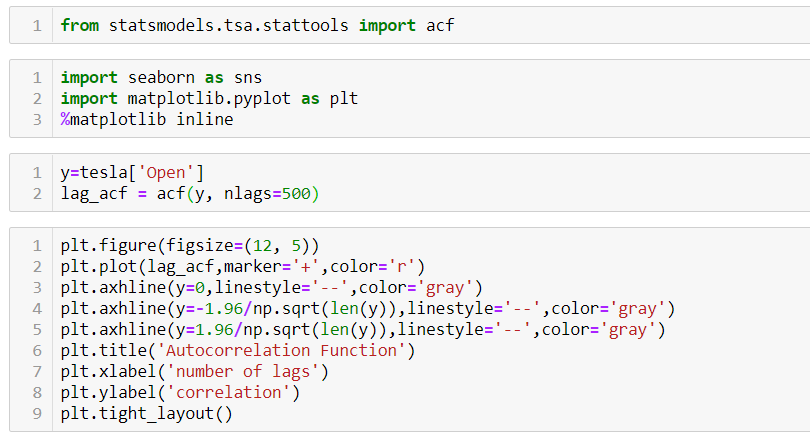
Using the stock price of tesla between the years 2012 and 2017 we can use the .acf() method in python to obtain the value of p.
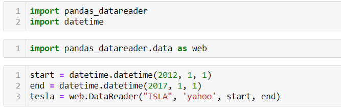
.DataReader() method is used to extract the data from web.

The above graph shows that beyond the lag 350 the correlation moved towards 0 and then negative.
PACF (Partial auto-correlation function) :- Pacf helps find the direct effect of the past lag by removing the residual effect of the lags in between. Pacf helps in obtaining the value of AR where as acf helps in obtaining the value of MA i.e. q. Both the methods together can be use find the optimum value of p and q in a time series data set.
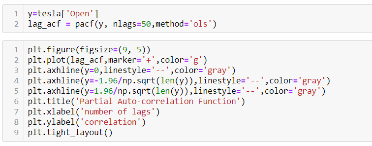
Lets check out how to apply pacf in python.
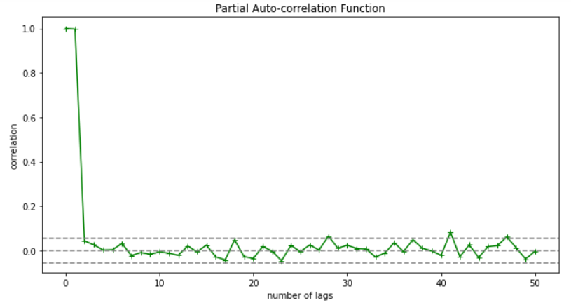
As you can see in the above graph after the second lag the line moved within the confidence band therefore the value of p will be 2.
So, with that we come to the end of the discussion on the ARMA Model. Hopefully it helped you understand the topic, for more information you can also watch the video tutorial attached down this blog. The blog is designed and prepared by Niharika Rai, Analytics Consultant, DexLab Analytics DexLab Analytics offers machine learning courses in Gurgaon. To keep on learning more, follow DexLab Analytics blog.
.
Advanced Analytics and Data Science, AI and Machine Learning, analytics training institute, Artificial Intelligence, artificial intelligence analytics, artificial intelligence certification, artificial intelligence training institute, Credit and Market Risk, Credit Risk, credit risk analysis, Credit Risk Analytics And Modeling, credit risk analytics training, Credit Risk Modelling, Credit Risk Modelling Using SAS, data science, Data Science Certification, Data Science Courses, data science online learning, Data Science training, Data Science training institute, deep learning certification, deep learning course, Deep Learning Training Courses, Deep learning Training Institutes, Machine Learning, Machine Learning Certification, Machine Learning course, Machine Learning course in Gurgaon, Machine Learning course online, Machine Learning Courses, Machine Learning Training, Machine Learning Using Python, Market Risk Analytics, market risk certification, market risk courses, Market Risk Management, Neural Networks Training, Online Data Science Certification, predictive analytics certification, python certification course, Python courses, python data science course, Python for data analysis, Python Training Institute
Comments are closed here.