
- Introduction
- What is Hypothesis Testing?
- Null Hypothesis, Alternative Hypothesis, Power of Test
- Type I and Type II Error
- Level of Significance, Critical Region
- Two-tailed and One-tailed test
- Solving Testing of Hypothesis Problem 8. Conclusion
- Conclusion
In this series we cover the basic of statistical inference, this is the fourth part of our discussion where we explain the concept of hypothesis testing which is a statistical technique. You could also check out the 3rd part of the series here.
Introduction
The objective of sampling is to study the features of the population on the basis of sample observations. A carefully selected sample is expected to reveal these features, and hence we shall infer about the population from a statistical analysis of the sample. This process is known as Statistical Inference.
There are two types of problems. Firstly, we may have no information at all about some characteristics of the population, especially the values of the parameters involved in the distribution, and it is required to obtain estimates of these parameters. This is the problem of Estimation. Secondly, some information or hypothetical values of the parameters may be available, and it is required to test how far the hypothesis is tenable in the light of the information provided by the sample. This is the problem of Test of Hypothesis or Test of Significance.
In many practical problems, statisticians are called upon to make decisions about a population on the basis of sample observations. For example, given a random sample, it may be required to decide whether the population, from which the sample has been obtained, is a normal distribution with mean = 40 and s.d. = 3 or not. In attempting to reach such decisions, it is necessary to make certain assumptions or guesses about the characteristics of population, particularly about the probability distribution or the values of its parameters. Such an assumption or statement about the population is called Statistical Hypothesis. The validity of a hypothesis will be tested by analyzing the sample. The procedure which enables us to decide whether a certain hypothesis is true or not, is called Test of Significance or Test of Hypothesis.
What Is Testing Of Hypothesis?
Statistical Hypothesis
Hypothesis is a statistical statement or a conjecture about the value of a parameter. The basic hypothesis being tested is called the null hypothesis. It is sometimes regarded as representing the current state of knowledge & belief about the value being tested. In a test the null hypothesis is constructed with alternative hypothesis denoted by 𝐻1 ,when a hypothesis is completely specified then it is called a simple hypothesis, when all factors of a distribution are not known then the hypothesis is known as a composite hypothesis.
Testing Of Hypothesis
The entire process of statistical inference is mainly inductive in nature, i.e., it is based on deciding the characteristics of the population on the basis of sample study. Such a decision always involves an element of risk i.e., the risk of taking wrong decisions. It is here that modern theory of probability plays a vital role & the statistical technique that helps us at arriving at the criterion for such decision is known as the testing of hypothesis.
Testing Of Statistical Hypothesis
A test of a statistical hypothesis is a two action decision after observing a random sample from the given population. The two action being the acceptance or rejection of hypothesis under consideration. Therefore a test is a rule which divides the entire sample space into two subsets.
- A region is which the data is consistent with 𝐻0.
- The second is its complement in which the data is inconsistent with 𝐻0.
The actual decision is however based on the values of the suitable functions of the data, the test statistic. The set of all possible values of a test statistic which is consistent with 𝐻0 is the acceptance region and all these values of the test statistic which is inconsistent with 𝐻0 is called the critical region. One important condition that must be kept in mind for efficient working of a test statistic is that the distribution must be specified.
Does the acceptance of a statistical hypothesis necessarily imply that it is true?
The truth a fallacy of a statistical hypothesis is based on the information contained in the sample. The rejection or the acceptance of the hypothesis is contingent on the consistency or inconsistency of the 𝐻0 with the sample observations. Therefore it should be clearly bowed in mind that the acceptance of a statistical hypothesis is due to the insufficient evidence provided by the sample to reject it & it doesn’t necessarily imply that it is true.
Elements: Null Hypothesis, Alternative Hypothesis, Pot
Null Hypothesis
A Null hypothesis is a hypothesis that says there is no statistical significance between the two variables in the hypothesis. There is no difference between certain characteristics of a population. It is denoted by the symbol 𝐻0. For example, the null hypothesis may be that the population mean is 40 then
𝐻0(𝜇 = 40)
Let us suppose that two different concerns manufacture drugs for including sleep, drug A manufactured by first concern and drug B manufactured by second concern. Each company claims that its drug is superior to that of the other and it is desired to test which is a superior drug A or B? To formulate the statistical hypothesis let X be a random variable which denotes the additional hours of sleep gained by an individual when drug A is given and let the random variable Y denote the additional hours to sleep gained when drug B is used. Let us suppose that X and Y follow the probability distributions with means 𝜇𝑥 and 𝜇𝑌 respectively.
Here our null hypothesis would be that there is no difference between the effects of two drugs. Symbolically,
𝐻0: 𝜇𝑋 = 𝜇𝑌
Alternative Hypothesis
A statistical hypothesis which differs from the null hypothesis is called an Alternative Hypothesis, and is denoted by 𝐻1. The alternative hypothesis is not tested, but its acceptance (rejection) depends on the rejection (acceptance) of the null hypothesis. Alternative hypothesis contradicts the null hypothesis. The choice of an appropriate critical region depends on the type of alternative hypothesis, whether both-sided, one-sided (right/left) or specified alternative.
Alternative hypothesis is usually denoted by 𝐻1.
For example, in the drugs problem, the alternative hypothesis could be
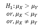
Power Of Test
The null hypothesis 𝐻0 𝜃 = 𝜃0 is accepted when the observed value of test statistic lies the critical region, as determined by the test procedure. Suppose that the true value of 𝜃 is not 𝜃0, but another value 𝜃1, i.e. a specified alternative hypothesis 𝐻1 𝜃 = 𝜃1 is true. Type II error is committed if 𝐻0 is not rejected, i.e. the test statistic lies outside the critical region. Hence the probability of Type II error is a function of 𝜃1, because now 𝜃 = 𝜃1 is assumed to be true. If 𝛽 𝜃1 denotes the probability of Type II error, when 𝜃 = 𝜃1 is true, the complementary probability 1 − 𝛽 𝜃1 is called power of the test against the specified alternative 𝐻1 𝜃 = 𝜃1 . Power = 1-Probability of Type II error=Probability of rejection 𝐻0 when 𝐻1 is true Obviously, we could like a test to be as ‘powerful’ as possible for all critical regions of the same size. Treated as a function of 𝜃, the expression of 𝑃 𝜃 = 1 − 𝛽 𝜃 is called Power Function of the test for 𝜃0 against 𝜃. the curve obtained by plotting P(𝜃) against all possible values of 𝜃, is known as Power Curve.
Elements: Type I & Type II Error
Type I Error & Type Ii Error
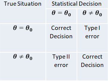
The procedure of testing statistical hypothesis does not guarantee that all decisions are perfectly accurate. At times, the test may lead to erroneous conclusions. This is so, because the decision is taken on the basis of sample values, which are themselves fluctuating and depend purely on chance. The errors in statistical decisions are two types:
- Type I Error – This is the error committed by the test in rejecting a true null hypothesis.
- Type II Error – This is the error committed by the test in accepting a false null hypothesis.
Considering for the population mean is 40, i.e. 𝐻0 𝜇 = 40 , let us imagine that we have a random sample from a population whose mean is really 40. if we apply the test for 𝐻0 𝜇 = 40 , we might find that the values of test statistic lines in the critical region, thereby leading to the conclusion that the population mean is not 40; i.e. the test rejects the null hypothesis although it is true. We have thus committed what is known as “Type I error” or “Error of first kind”. On the other hand, suppose that we have a random sample from a population whose mean is known to different from 40, say 43. if we apply the test for 𝐻0 𝜇 = 40 , the value of the statistic may, by chance, lie in the acceptance region, leading to the conclusion that the mean may be 40; i.e. the test does not reject the null hypothesis 𝐻0 𝜇 = 40 , although it is false. This is again another form of incorrect decision, and the error thus committed is known as “Type II error” or “Error of second kind”.
 Using sampling distribution of the test statistic, we can measure in advance the probabilities of committing the two types of error. Since the null hypothesis is rejected only when the test statistic falls in the critical region.
Probability of Type I error = Probability of rejecting 𝐻0 𝜃 = 𝜃0 , when it is true
= Probability that the test statistic lies in the critical region, assuming 𝜃 = 𝜃0.
The probability of Type I error must not exceed the level of significance (𝛼) of the test.
𝑃𝑟𝑜𝑏𝑎𝑏𝑖𝑙𝑖𝑡𝑦 𝑜𝑓 𝑇𝑦𝑝𝑒 𝐼 𝑒𝑟𝑟𝑜𝑟 ≤ 𝐿𝑒𝑣𝑒𝑙 𝑜𝑓 𝑆𝑖𝑔𝑛𝑖𝑓𝑖𝑐𝑎𝑛𝑐𝑒
The probability of Type II error assumes different values for different values of 𝜃 covered by the alternative hypothesis 𝐻1. Since the null hypothesis is accepted only when the observed value of the best statistic lies outside the critical region.
Probability of Type II error 𝑊ℎ𝑒𝑛 𝜃 = 𝜃1
= Probability of accepting 𝐻0 𝜃 = 𝜃0 , when it is false
= Probability that the test statistic lies in the region of acceptance, assuming 𝜃 = 𝜃1
The probability of Type I error is necessary for constructing a test of significance. It is in fact the ‘size of the Critical Region’. The probability of Type II error is used to measure the “power” of the test in detecting falsity of the null hypothesis. When the population has a continuous distribution
Probability of Type I error
= Level of significance
= Size of critical region
Elements: Level Of Significance & Critical Region
Level Of Significance And Critical Region
The decision about rejection or otherwise of the null hypothesis is based on probability considerations. Assuming the null hypothesis to be true, we calculate the probability of obtaining a difference equal to or greater than the observed difference. If this probability is found to be small, say less than .05, the conclusion is that the observed value of the statistic is rather unusual and has been caused due to the underlying assumption (i.e. null hypothesis) that is not true. We say that the observed difference is significant at 5 per cent level, and hence the ‘null hypothesis is rejected’ at 5 per cent level of significance. If, however, this probability is not very small, say more than .05, the observed difference cannot be considered to be unusual and is attributed to sampling fluctuation only. The difference is, now said to be not significant at 5 per cent level, and we conclude that there is no reason to reject the null hypothesis’ at 5 per cent level of significance. It has become customary to use 5% and 1% level of significance, although other levels, such as 2% or 5% may also be used.
Without actually going to calculate this probability, the test of significance may be simplified as follows. From the sampling distribution of the statistic, we find the maximum difference is which is exceeded in (say 5) percent of cases. If the observed difference in larger than this value, the null hypothesis is rejected. It is less there in no reason to reject the null hypothesis.
Suppose, the sampling distribution of the statistic is a normal distribution. Since the area under normal curve outside the ordinates at mean ±1.96 (𝑠. 𝑑. ) is only 5%, the probability that the observed value of the statistic differs from the expected value of 1.96 times the S.E. or more is .05; and the probability of a larger difference will be still smaller. If, therefore
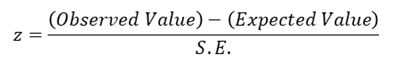
Is either greater than 1.96 or less than -1.96 (i.e. numerically greater than 1.96), the null hypothesis 𝐻0 is rejected at 5% level of significance. The set values 𝑧 ≥ 1.96 𝑜𝑟 ≤ −1.96, i.e.
|𝑧| ≥ 1.96
constitutes what is called the Critical Region for the test. Similarly since the area outside mean ±2.58 (s.d.) is only 1%. 𝐻0 is rejected at 1% level of significance, if z numerically exceeds 258, i.e. the critical region is 𝑧 ≥ 2.58 at 1% level. Using the sampling distribution of an appropriate test statistic we are able to establish the maximum difference at a specified level between the observed and expected values that is consistent with null hypothesis 𝐻0 . The set of values of the test statistic corresponding to this difference which lead to the acceptance of 𝐻0 is called Region of acceptance. Conversely, the set of values of the statistic leading to the rejection of 𝐻0 is referred to as Region of Rejection or “Critical Region” of the test. The value of the statistic which lies at the boundary of the regions of acceptance and the rejection is called Critical value. When the null hypothesis is true, the probability of observed value of the test statistic falling in the critical region is often called the “Size of Critical Region”.
𝑆𝑖𝑧𝑒 𝑜𝑓 𝐶𝑟𝑖𝑡𝑖𝑐𝑎𝑙 𝑅𝑒𝑔𝑖𝑜𝑛 ≤ 𝐿𝑒𝑣𝑒𝑙 𝑜𝑓 𝑆𝑖𝑔𝑛𝑖𝑓𝑖𝑐𝑎𝑛𝑐𝑒
However, for a continuous population, the critical region is so determined that its size equals the Level of Significance (𝛼).
Two-Tailed And One-Tailed Tests
Our discussion above were centered around testing the significance of ‘difference’ between the observed and expected values, i.e. whether the observed value is significantly different from (i.e. either larger or smaller than) the expected value, as could arise due to fluctuations of random sampling. In the illustration, the null hypothesis is tested against “both-sided alternatives” 𝜇 > 40 𝑜𝑟 𝜇 < 40 , i.e.
𝐻0 𝜇 = 40 𝑎𝑔𝑎𝑖𝑛𝑠𝑡 𝐻1 𝜇 ≠ 40
Thus assuming 𝐻0 to be true, we would be looking for large differences on both sides of the expected value, i.e. in “both tails” of the distribution. Such tests are, therefore, called “Two-tailed tests”.
Sometimes we are interested in tests for large differences on one side only i.e., in one ‘one tail’ of the distribution. For example, whether a change in the production bricks with a ‘higher’ breaking strength, or whether a change in the production technique yields ‘lower’ percentage of defectives. These are known as “One-tailed tests”.
For testing the null hypothesis against “one-sided alternatives (right side)” 𝜇 > 40 , i.e.
𝐻0 𝜇 = 40 𝑎𝑔𝑎𝑖𝑛𝑠𝑡𝐻1 𝜇 > 40
The calculated value of the statistic z is compared with 1.645, since 5% of the area under the standard normal curve lies to the right of 1.645. if the observed value of z exceeds 1.645, the null hypothesis 𝐻0 is rejected at 5% level of significance. If a 1% level were used, we would replace 1.645 by 2.33. thus the critical regions for test at 5% and 1% levels are 𝑧 ≥ 1.645 and 𝑧 ≥ 2.33 respectively.
For testing the null hypothesis against “one-sided alternatives (left side)” 𝜇 < 40 i.e.
𝐻0 𝜇 = 40 𝑎𝑔𝑎𝑖𝑛𝑠𝑡𝐻1 𝜇 < 40
The value of z is compared with -1.645 for significance at 5% level, and with -2.33 for significance at 1% level. The critical regions are now 𝑧 ≤ −1.645 and 𝑧 ≤ −2.33 for 5% and 1% levels respectively. In fact, the sampling distributions of many of the commonly-used statistics can be approximated by normal distributions as the sample size increases, so that these rules are applicable in most cases when the sample size is ‘large’, say, more than 30. It is evident that the same null hypothesis may be tested against alternative hypothesis of different types depending on the nature of the problem. Correspondingly, the type of test and the critical region associated with each test will also be different.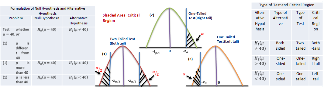
Solving Testing Of Hypothesis Problem
Step 1
Set up the “Null Hypothesis” 𝐻0 and the “Alternative Hypothesis” 𝐻1 on the basis of the given problem. The null hypothesis usually specifies the values of some parameters involved in the population: 𝐻0 𝜃 = 𝜃0 . The alternative hypothesis may be any one of the following types: 𝐻1 ( ) 𝜃 ≠ 𝜃1 𝐻1 𝜃 > 𝜃0 , 𝐻1 𝜃 < 𝜃0 . The types of alternative hypothesis determines whether to use a two-tailed or one-tailed test (right or left tail).
Step 2
State the appropriate “test statistic” T and also its sampling distribution, when the null hypothesis is true. In large sample tests the statistic 𝑧 = (𝑇 − 𝜃0)Τ𝑆. 𝐸. , (T) which approximately follows Standard Normal Distribution, is often used. In small sample tests, the population is assumed to be Normal and various test statistics are used which follow Standard Normal, Chi-square, t for F distribution exactly.
Step 3
Select the “level of significance” 𝛼 of the test, if it is not specified in the given problem. This represents the maximum probability of committing a Type I error, i.e., of making a wrong decision by the test procedure when in fact the null hypothesis is true. Usually, a 5% or 1% level of significance is used (If nothing is mentioned, use 5% level).
Step 4
Find the “Critical region” of the test at the chosen level of significance. This represents the set of values of the test statistic which lead to rejection of the null hypothesis. The critical region always appears in one or both tails of the distribution, depending on weather the alternative hypothesis is one-sided or both-sided. The area in the tails must be equal to the level of significance 𝛼. For a one-tailed test, 𝛼 appears in one tail and for two-tailed test 𝛼/2 appears in each tail of the distribution. The critical region is
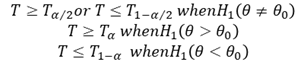
Where 𝑇𝛼 is the value of T such that the area to its tight is 𝛼.
Step 5
Compute the value of the test statistic T on the basis of sample data the null hypothesis. In large sample tests, if some parameters remain unknown they should be estimated from the sample.
Step 6
If the computed value of test statistic T lies in the critical region, “reject 𝐻0”; otherwise “do not reject 𝐻0 ”. The decision regarding rejection or otherwise of 𝐻0 is made after a comparison of the computed value of T with critical value (i.e., boundary value of the appropriate critical region).
Step 7
Write the conclusion in plain non-technical language. If 𝐻0 is rejected, the interpretation is: “the data are not consistent with the assumption that the null hypothesis is true and hence 𝐻0 is not tenable”. If 𝐻0 is not rejected, “the data cannot provide any evidence against the null hypothesis and hence 𝐻0 may be accepted to the true”. The conclusion should preferably be given in the words stated in the problem.
Conclusion
Hypothesis is a statistical statement or a conjecture about the value of a parameter. The legal concept that one is innocent until proven guilty has an analogous use in the world of statistics. In devising a test, statisticians do not attempt to prove that a particular statement or hypothesis is true. Instead, they assume that the hypothesis is incorrect (like not guilty), and then work to find statistical evidence that would allow them to overturn that assumption. In statistics this process is referred to as hypothesis testing, and it is often used to test the relationship between two variables. A hypothesis makes a prediction about some relationship of interest. Then, based on actual data and a pre-selected level of statistical significance, that hypothesis is either accepted or rejected. There are some elements of hypothesis like null hypothesis, alternative hypothesis, type I & type II error, level of significance, critical region and power of test and some processes like one and two tail test to find the critical region of the graph as well as the error that help us reach the final conclusion.
A Null hypothesis is a hypothesis that says there is no statistical significance between the two variables in the hypothesis. There is no difference between certain characteristics of a population. It is denoted by the symbol 𝐻0. A statistical hypothesis which differs from the null hypothesis is called an Alternative Hypothesis, and is denoted by 𝐻1. The procedure of testing statistical hypothesis does not guarantee that all decisions are perfectly accurate. At times, the test may lead to erroneous conclusions. This is so, because the decision is taken on the basis of sample values, which are themselves fluctuating and depend purely on chance, this process called types of error. Hypothesis testing is very important part of statistical analysis. By the help of hypothesis testing many business problem can be solved accurately.
That was the fourth part of the series, that explained hypothesis testing and hopefully it clarified your notion of the same by discussing each crucial aspect of it. You can find more informative posts like this one on Data Science course topics. Just keep on following the Dexlab Analytics blog to stay informed.
.
Business analysis training, business analytics, business analytics certification, business analytics course in delhi, Business Analytics Online, Business Analytics Online Certification, data science, Data Science Certification, Data Science Classes, Data Science Courses, data science online learning, Data Science training
Comments are closed here.