How to Append Data to Add Markers to SAS Graphs

Would you like to create customized SAS graphs with the use of PROC SGPLOT and other ODS graphic procedures? Then an essential skill that you must learn is to know how to join, merge, concentrate and append SAS data sets, which arise from a variety of sources. The SG procedures, which stand for SAS statistical graphic procedures, enable users to overlay different kinds of customized curves, bars and markers. But the SG procedures do expect all the data for a graph to be in one single set of data. Thus, it often becomes necessary to append two or more sets of data before one can create a complex graph.

In this blog post, we will discuss two ways in which we can combine data sets in order to create ODS graphics. An alternative option is to use the SG annotation facility, which will add extra curves and markers to the graph. We mostly recommend the use of the techniques that are given in this article for simple features and reserve annotations when adding highly complex yet non-standard features.

Using overlay curves:

Here is a brief idea on how to structure a SAS data set, so that one can overlay curves on a scatter plot.

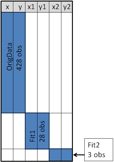
The original data is contained in the X and Y variables, as can be seen from the picture below. These will be the coordinates for the scatter plot. The secondary information will be appended at the end of the data. The variables X1 and Y1 contain the coordinates of a custom scatter plot smoother. The X2 and Y2 variables contain the coordinates of another scatter plot smoother.

Source: blogs.sas.com

This structure will enable you to use the SGPLOT procedure for overlaying, two curves on the scatter plot. One may make use of a SCATTER statement along with two SERIES statements to build the graphs.

With the right Retail Analytics Courses, you can learn to do the same, and much more with SAS.

Using Overlay Markers: Wide form

Sometimes in addition to the overlaying curves, we like to add special markers to the scatter plot. In this blog we plan to show people how to add a marker that shows the location of the sample mean. It will discuss how to use PROC MEANS to build an output data set, which contains the coordinates of the sample mean, then we will append the data set to the original data.

With the below mentioned statements we can use PROC MEANS for computing the sample mean of the four variables in the data set of SasHelp.Iris. This data contains the measurements for 150 iris flowers. To further emphasize on the general syntax of this computation, we will make use of macro variables but note that it is not necessary:

%let DSName = Sashelp.Iris;
%let VarNames = PetalLength PetalWidth SepalLength SepalWidth;
  
proc means data=&DSName noprint;
var &VarNames;
output out=Means(drop=_TYPE_ _FREQ_) mean= / autoname;
run;

With the AUTONAME option on the output statement, we can tell PROC MEANS to append the name of the statistics to names of the variables. As a result, the output datasets will contain the variables, with names like PetalLength_Mean or SepalWidth_Mean.

As depicted in the previous picture, this will enable you to append the new data into the end of the old data in the “wide form”, as shown here:

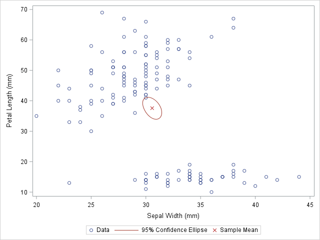
data Wide;
   set &DSName Means; /* add four new variables; pad with missing values */
run;
 
ods graphics / attrpriority=color subpixel;
proc sgplot data=Wide;
scatter x=SepalWidth y=PetalLength / legendlabel="Data";
ellipse x=SepalWidth y=PetalLength / type=mean;
scatter x=SepalWidth_Mean y=PetalLength_Mean / 
         legendlabel="Sample Mean" markerattrs=(symbol=X color=firebrick);
run;

And as here:

Source: blogs.sas.com

The original data is used in the first SCATTER statement and the ELLIPSE statement. You must remember that the ELLIPSE statement draws an approximate confidence ellipse for the population mean. The second SCATTER statement also makes use of sample means, which must be appended to the end of the original data. The second SCATTER statement will draw a red marker at the location of the sample mean.

This method can be used to plot other sample statistics (like the median) or to highlight special values such as the origin of a coordinate system.

Using overlay markers: of the long form

In certain circumstances, it is better to append the secondary data in the “long form”. In the long form the secondary data sets contains variables similar to the names in the original data set. One can choose to use the SAS data step to build a variable that will pinpoint the original and supplementary observations. With this technique it will be useful when people would want to show multiple markers (like, sample, mean, median, mode etc.) by making use of the GROUP = option on one of the SCATTER statement.

For detailed explanation of these steps and more on such techniques, join our SAS training courses in Delhi.

The following call to the PROC MEANS does not make use of an AUTONAME option. That is why the output data sets contain variables which have the same name as the input data. One can make use of the IN= data set option, for creating the ID variables that identifies with the data from the computed statistics:

/* Long form. New data has same name but different group ID */
proc means data=&DSName noprint;
var &VarNames;
output out=Means(drop=_TYPE_ _FREQ_) mean=;
run;
 
data Long;
set &DSName Means(in=newdata);
if newdata then 
   GroupID = "Mean";
else GroupID = "Data";
run;

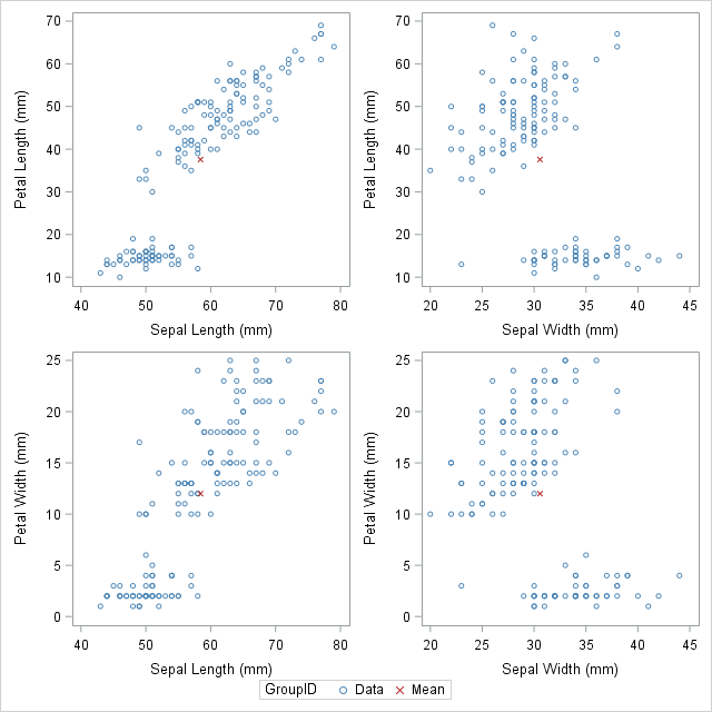
The DATA step is used to create the GroupID variable, which has several values “Data” for the original observations and the value “Mean” for the appended observations. This data structure will be useful for calling the PROC SGSCATTER and this will support the GROUP = option, however it does not support multiple PLOT statements as the following:

ods graphics / attrpriority=none;
proc sgscatter data=Long 
   datacontrastcolors=(steelblue firebrick)
   datasymbols=(Circle X);
plot (PetalLength PetalWidth)*(SepalLength SepalWidth) / group=groupID;
run;

Source: blogs.sas.com

In closing thoughts, this blog is to demonstrate some useful techniques, to add markers to a graph. The technique requires people to use concatenate the original data with supplementary data. Often for creating ODS statistical graphics it is better to use appending and merging data technique in SAS. This is a great technique to include in your programming capabilities.

SAS courses in Noida can give you further details on some more techniques that are worth adding to your analytics toolbox!

 
This post originally appeared on – blogs.sas.com/content/iml/2016/11/30/append-data-add-markers-sas-graphs.html
 

Interested in a career in Data Analyst?

To learn more about Data Analyst with Advanced excel course – Enrol Now.
To learn more about Data Analyst with R Course – Enrol Now.
To learn more about Big Data Course – Enrol Now.

To learn more about Machine Learning Using Python and Spark – Enrol Now.
To learn more about Data Analyst with SAS Course – Enrol Now.
To learn more about Data Analyst with Apache Spark Course – Enrol Now.
To learn more about Data Analyst with Market Risk Analytics and Modelling Course – Enrol Now.